Answer
- Open the “Data” tab and select “Sheets.”
- In the “Sheets” window, click on the “Graphs” tab and select the graph you want to modify.
- Under “Axes,” select the axis you want to change the color of.
- Then, under “Color,” select a new color.
How to Change the Bar Colour in Google Sheets Bar Graph
Change chart border color in Google Sheets
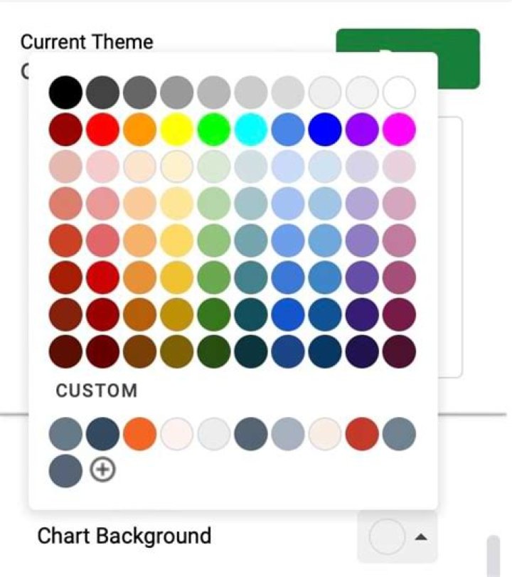
How do you change the grid color in Google Sheets?To change the grid color in Google Sheets, open the “Sheets” app on your phone or computer, click on the “File” menu, and select “Make a copy…” Then select the “Sheet” you want to modify and click on the “Make changes” button. In the “Colors” tab, select the color you want for your grid lines and click on the “OK” button.
How do I change the color of my graph?There are a few ways to change the color of your graph:
-Select the “Customize Graph” button in the toolbar and select the “Color” option.
-Select the “Plot” tab and select the “Color” option.
-Select the legend item and choose a different color.
There are a few ways to customize a graph in Google Sheets:
-Select the data you want to graph and click “Add Data Series.”
-Click “Customize Graph” on the toolbar and select the data you want to graph.
-Click “Layout” on the toolbar and select a layout for your graph.
To change the theme on a graph in Google Sheets, follow these steps:
Open the graph you want to customize in Google Sheets.
Click the “Theme” button in the toolbar at the top of the sheet.
Select a new theme from the list.
Click OK to apply the theme.
There are a few ways to make charts look beautiful in Google Sheets. One way is to use color coding to differentiate different data sets. For example, you could use green for data that is positive, yellow for data that is neutral, and red for data that is negative. Another way to make charts look beautiful is to add borders around the chart. You can also add shading and highlights to your charts to make them more visually appealing.
How do I change the legend color in Excel?To change the legend color in Excel, follow these steps:
Open Excel and select the data you want to modify.
Click on the Data tab and then click on the Legend icon.
Select the color you want for the legend in the Legend Color box.
There are a few ways to change the color of your bar chart based on value. One way is to use a categorical color scale, which assigns different colors to different values. For example, you could use green for values between $0 and $10, yellow for values between $10 and $20, and red for values over $20. Another way is to use a gradient color scale, which starts with one color and gradually transitions to another color as the value increases.
How do you change the color of a line graph in Excel?There are a few ways to change the color of a line graph in Excel. One way is to use the Color palette, which can be found in the Home tab of the ribbon. Another way is to use the Line tool and select a new color from the palette.
How do you make a multi colored bar graph in Excel?There are a few ways to make a multi-colored bar graph in Excel. One way is to use the VLOOKUP function. You can also use the AVERAGE function to calculate the average color for each group.
How do you change the color of a line in Google Docs?To change the color of a line in Google Docs, open the document and click on the pencil icon in the top left corner. From the drop-down menu that appears, select “Line Color.” You can then select a different color from the list.
How do I get rid of the black outline in Google Sheets?There are a few ways to fix the black outline issue on Google Sheets. The easiest way is to use the “Highlighter” tool in the “Tools” menu. Select the cells that need to be highlighted, and then click on the “Highlighter” button. This will allow you to change the color of the border around the highlighted cells. Another option is to use the “Filter” tool.
How do I make Google Docs darker?To make Google Docs darker, you can either change the color scheme or use a dark theme.
How do I make Google Sheets visually appealing?There are a few things that you can do to make your Google Sheets look more appealing. First, make sure that the font size is large enough so that all of the text is readable. Second, try to use a color scheme that is both eye-catching and functional. Finally, make sure that all of the data is easily accessible by using tabs or column headings.
How do you make a chart look good on Google Docs?There are a few things you can do to make your charts look good on Google Docs. First, make sure that the chart is formatted correctly. You can format your chart using the formatting options in the editor toolbar or by using the Chart Tools menu. You can also use the Chart Type menu to change the type of chart you’re creating.
Another way to make your charts look good on Google Docs is to use color and fonts.
There are a few ways to create a multiple bar graph in Google Sheets. The easiest way is to use the VLOOKUP function. To create a graph with three bars, use the following code:
=VLOOKUP(A2,Sheet1!$A$2:$D$2,3)
The VLOOKUP function will return the value of the cell located at the intersection of the two columns that match the search criteria.
